Bosonic Environments

The basic class object used to construct the problem is imported in the following way (alongside QuTiP, with which we define system Hamiltonian and coupling operators)

from qutip import *
from bofin.heom import BosonicHEOMSolver

If one is using the C++ BoFiN_fast package, the import is instead

from qutip import *
from bofinfast.heom import BosonicHEOMSolver

Apart from this difference in import, and some additional features in the solvers in the C++ variant, the functionality that follows applies to both libraries.

One defines a particular problem instance in the following way:

Solver = BosonicHEOMSolver(Hsys, Q, ckAR, ckAI, vkAR, vkAI, NC, options=options)

The parameters accepted by the solver are : - Hsys : the system Hamiltonian in quantum object form - Q a coupling operator (or list of coupling operators) that couple the system to the environment - ckAR and vkAR : respectively the coefficients and frequencies of the real parts of the correlation functions - ckAI and vkAI : respectively the coefficients and frequencies of the imaginary parts of the correlation functions - NC : the truncation parameter of the hierarchy - options is a standard QuTiP ODEoptions object, which is used by the ODE solver.

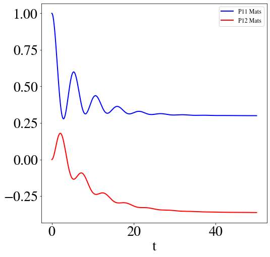
Thus an example solution to a single spin coupled to a Drude-Lorentz spectral density with Matsubara decomposition is (taken from example notebook 1a):

%pylab inline
from qutip import *
from bofin.heom import BosonicHEOMSolver

def cot(x):
    return 1./np.tan(x)

    # Defining the system Hamiltonian
eps = .5     # Energy of the 2-level system.
Del = 1.0    # Tunnelling term
Hsys = 0.5 * eps * sigmaz() + 0.5 * Del* sigmax()

    # Initial state of the system.
rho0 = basis(2,0) * basis(2,0).dag()

    # System-bath coupling (Drude-Lorentz spectral density)
Q = sigmaz() # coupling operator

tlist = np.linspace(0, 50, 1000)

    #Bath properties:
gamma = .5 # cut off frequency
lam = .1 # coupling strength
T = 0.5
beta = 1./T

    #HEOM parameters
NC = 5 # cut off parameter for the bath
Nk = 2 # number of Matsubara terms
ckAR = [ lam * gamma * (cot(gamma / (2 * T)))]
ckAR.extend([(4 * lam * gamma * T *  2 * np.pi * k * T / (( 2 * np.pi * k * T)**2 - gamma**2)) for k in range(1,Nk+1)])
vkAR = [gamma]
vkAR.extend([2 * np.pi * k * T for k in range(1,Nk+1)])
ckAI = [lam * gamma * (-1.0)]
vkAI = [gamma]
NR = len(ckAR)
NI = len(ckAI)
Q2 = [Q for kk in range(NR+NI)]


options = Options(nsteps=15000, store_states=True, rtol=1e-14, atol=1e-14)
HEOMMats = BosonicHEOMSolver(Hsys, Q2, ckAR, ckAI, vkAR, vkAI, NC, options=options)

    #Run ODE solver
resultMats = HEOMMats.run(rho0, tlist)

# Define some operators with which we will measure the system
# Populations
P11p=basis(2,0) * basis(2,0).dag()
P22p=basis(2,1) * basis(2,1).dag()
# 1,2 element of density matrix  - corresonding to coherence
P12p=basis(2,0) * basis(2,1).dag()
# Calculate expectation values in the bases
P11exp = expect(resultMats.states, P11p)
P22exp = expect(resultMats.states, P22p)
P12exp = expect(resultMats.states, P12p)

# Plot the results
fig, axes = plt.subplots(1, 1, sharex=True, figsize=(8,8))
axes.plot(tlist, np.real(P11exp), 'b', linewidth=2, label="P11 Mats")
axes.plot(tlist, np.real(P12exp), 'r', linewidth=2, label="P12 Mats")
axes.set_xlabel(r't', fontsize=28)
axes.legend(loc=0, fontsize=12)

Multiple environments

The above example describes a single environment parameterized by the lists of coefficients and frequencies in the correlation functions.

For multiple environments, the list of coupling operators and bath properties must all be extended in a particular way. Note this functionality differs in the case of the Fermionic solver.

For the Bosonic solver, for N baths, each ckAR, vkAR, ckAI, and vkAI are extended N times with the appropriate number of terms of that bath.

On the other hand, the list of coupling operators is defined in such a way that the terms corresponding to the real cooefficients are given first, and the imaginary terms after. Thus if each bath has \(N_k\) coefficients, the list of coupling operators is of length \(N_k \times (N_R + N_I)\).

This is best illustrated by the example in example notebook 2. In that case each bath is identical, and there are seven baths, each with a unique coupling operator defined by a projector onto a single state:

ckAR = [pref * lam * gamma * (cot(gamma / (2 * T))) + 0.j]
ckAR.extend([(pref * 4 * lam * gamma * T *  2 * np.pi * k * T / (( 2 * np.pi * k * T)**2 - gamma**2))+0.j for k in range(1,Nk+1)])
vkAR = [gamma+0.j]
vkAR.extend([2 * np.pi * k * T + 0.j for k in range(1,Nk+1)])
ckAI = [pref * lam * gamma * (-1.0) + 0.j]
vkAI = [gamma+0.j]

NR = len(ckAR)
NI = len(ckAI)
Q2 = []
ckAR2 = []
ckAI2 = []
vkAR2 = []
vkAI2 = []
for m in range(7):
    Q2.extend([ basis(7,m)*basis(7,m).dag() for kk in range(NR)])
    ckAR2.extend(ckAR)
    vkAR2.extend(vkAR)

for m in range(7):
    Q2.extend([ basis(7,m)*basis(7,m).dag() for kk in range(NI)])
    ckAI2.extend(ckAI)
    vkAI2.extend(vkAI)